
Why Transformer Architecture Choice Defines LLM Inference Cost, Latency, and Scale

Your team has a working LLM prototype, and the model choice that suited a handful of testers now has to survive production traffic. A larger model, a quantized model, and a retrieval-augmented setup all look reasonable on paper.
Each option changes LLM inference, the work of running a trained model on a prompt, by changing the memory and time each request needs. A model that runs well for one tester might exhaust GPU memory, because every concurrent request holds memory until its last token. It might also miss your latency target or exceed your budget.
This guide shows you how to estimate GPU memory for a 13B model, split latency into prefill and decode, and measure a serving setup. You finish with a checklist for reviewing your own deployment.
Why LLM inference decisions start with architecture
LLM inference is the step that turns input tokens into output tokens, which makes it the part of your system that users wait on. According to Modular's inference handbook, training builds the model once, while inference runs every time a user sends a request. Inference therefore sets the cost that grows with your traffic.
A large language model (LLM) is a neural network trained on text to predict the next token. At the core of most LLMs lies a transformer that generates one token at a time. An LLM is the trained model and inference is the act of running it, so ChatGPT performs inference whenever it answers a message.
Parameter count is only one input to your deployment decision, because precision, context length, and request concurrency matter as well. The sections below move from memory to precision, then to retrieval and serving.
Model size and its impact on cost and latency
Model size sets the first hard limit on your hardware, because every parameter must sit in GPU memory. Parameter count and numeric precision therefore decide how much memory the weights need.
You can estimate that memory by multiplying the parameter count by the bytes each parameter uses. A 13B model in FP16 stores each parameter in two bytes, so the weights need about 26 GB.
Model-weight memory ≈ parameter count × bytes per parameter

13B parameters × 2 bytes for FP16
≈ 26 GB for model weights
The vLLM paper lists the same 26 GB for a 13B model. That figure covers only the weights and leaves out four other memory costs:
- The KV cache, the attention state that each request adds
- Activations
- Runtime overhead
- Operational headroom
More weights need more GPU memory, and a model split across GPUs must also synchronize results between them, which adds communication work to every step. Mistral AI's own evaluation shows Mistral 7B outperforming Llama 2 13B on all reported benchmarks, so a larger model must earn its memory.
What LLM inference does during a request
A request starts as text, and the model splits it into tokens before running them through transformer layers. The model then generates output tokens one at a time, and each new token depends on all the ones before it.
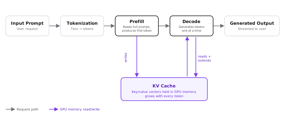
The vLLM paper splits a request into two phases, starting with a prompt phase that reads all input tokens together. That phase produces the first output token, a step the paper also calls prefill.
In the generation phase, the model produces the remaining tokens sequentially. This decode phase is memory-bound, meaning data movement limits its speed, so it underuses GPU compute. According to the paper, it accounts for most of a single request's latency.
Databricks ties time to first token (TTFT) to processing the prompt and producing the first token. It ties time per output token (TPOT) to each token after that.
The two phases call for different fixes, because prefill work grows with prompt length and decode work grows with output length. The diagram below maps each phase onto the request path.
Why model size is only the first memory calculation
Weights stay fixed while the model serves requests, but each request adds state of its own. That state is the KV cache, which stores the key and value vectors that the attention mechanism computes for earlier tokens.
Without the cache, the model would recompute those vectors for every earlier token at every step. With the cache, the model computes only the newest token's vectors and reads the rest from memory.
The cache grows with every token, so you can estimate its size from the model's shape. The vLLM paper multiplies four numbers to get the per-token cost for a 13B model.
KV cache per token ≈ 2 (keys and values) × hidden size × layers × bytes per value

2 × 5,120 × 40 × 2 bytes (FP16)
≈ 0.8 MB per token

0.8 MB × 2,048 tokens
≈ 1.6 GB for one request
These figures come from the paper's OPT-13B example. NVIDIA's inference optimization guide gives the same formula for per-token cache size. A Llama 2 13B-shaped model has the same 40 layers and 5,120 hidden size, so it gives the same estimate. Real memory use depends on six factors:
- Architecture
- Precision
- Sequence length
- Batching
- Implementation
- Runtime overhead
The general formula replaces the hidden size with the number of key-value heads times the head dimension. Models with fewer key-value heads therefore store less per token. Sebastian Raschka's calculator lists 144 KiB per token for Qwen3 8B.
Memory multiplies with concurrency because every active request needs its own cache. In the paper's setup, a 40 GB A100 devotes 26 GB to weights and 12 GB to the KV cache. That cache space fits about 15,700 tokens across all active requests. By that arithmetic, fewer than eight requests of 2,048 tokens fit at once, so cache memory caps your batch size.
Precision, quantization, and inference efficiency
Precision sets how many bytes each stored number uses. FP16 uses two bytes and INT8 uses one, so moving the weights from FP16 to INT8 halves their memory.
Quantization converts a model to a lower precision, which can let it fit on fewer GPUs. The change also alters the arithmetic, so the outputs might change.
The table applies the same bytes-per-parameter arithmetic to a 13B model. It excludes the KV cache and runtime overhead, so treat the numbers as a floor.
| Precision | Bytes per parameter | Weight memory |
|---|---|---|
| FP16 | 2 | 26 GB |
| INT8 | 1 | 13 GB |
| INT4 | 0.5 | 6.5 GB |
Lower memory doesn't guarantee a faster or cheaper deployment, because speed depends on hardware, runtime, and workload shape. NVIDIA TensorRT lists INT8 and FP16 optimizations, but only a test on your own workload shows whether they help.
Precision also affects concurrency, because memory freed from weights leaves room for the KV cache. The vLLM paper ties the number of batched requests to that space.
What to measure after changing precision
Treat a precision change as an experiment. Keep the prompts, the hardware, and the serving configuration constant, so any change in the results comes from the precision alone. Record four results for each precision:
- Task quality on your own prompts, before and after the change
- TTFT, TPOT, and total generation time
- Throughput and GPU memory use
- Workload mix of prefill-heavy and decode-heavy requests
If quality drops after quantization, then test the workload with task-specific evaluations. Parameter count alone won't tell you which model holds up.
Retrieval and serving setup for scalable SaaS deployments
Retrieval-augmented generation (RAG), introduced by Lewis et al. in 2020, combines a model with an external index of documents. Serving decisions then determine how the longer prompts share your GPUs.
Retrieval changes the shape of inference work
RAG retrieves documents at request time and adds them to the prompt. The RAG paper reports more factual output than a baseline that lacks retrieval. Every retrieved chunk also becomes input tokens that the model must process.
Compare a short prompt with a retrieval-augmented prompt that carries many extra tokens. The longer prompt raises prefill work and adds KV cache for every request that uses it.
Measure retrieval depth, time to first token, and answer quality together. Retrieval adds tokens, which might raise both cost and latency.
Batching and caching change utilization
Batching processes several requests together so the GPU spends less time idle. It's hard to do well, because the vLLM paper notes that requests arrive at different times and a naive policy makes early requests wait.
Batching can raise throughput while it adds queueing delay for individual requests. Compare throughput and per-request latency separately before changing a batching policy.
Caching lets the model skip work it already did. The vLLM paper describes storing the KV cache of a shared prefix, such as a system prompt, so each request computes only its own input. As of September 2026, OpenAI lists cached input for gpt-6-astra at $1.00 per million tokens, against $10.00 for uncached input. Check your runtime's documentation to learn what it caches and for how long.
Choose serving infrastructure against the workload
Your serving choice comes down to the controls you need and who owns operations, since each option shifts both. Compare your options on six operating factors:
- Model loading time
- Autoscaling behavior
- GPU availability
- Observability
- Batching controls
- Operational ownership
A managed endpoint hands most operations to a provider. Amazon SageMaker AI multi-model endpoints, for example, host many models on shared resources. They load each model into memory on demand, so the first request to a model takes longer.
An inference server runs models on infrastructure you control. NVIDIA Triton Inference Server runs multiple models concurrently and applies dynamic batching to improve throughput, according to its README.
A serving framework adds LLM-specific features, and Ray Serve lists response streaming, dynamic request batching, and multi-node, multi-GPU serving for LLMs. In the authors' evaluation, vLLM reaches two to four times the throughput of FasterTransformer and Orca at the same latency.
A custom deployment gives you the most control and the most work, because you build and run every layer yourself. None of these options fits every workload, so match the choice to your traffic and your team.
How to measure LLM inference before production
Parameter count won't tell you how a deployment performs, so measure LLM inference with your own prompts and your target hardware. Inference optimization starts from your own data, because only your workload shows what consumes time and memory.
Total latency equals TTFT plus TPOT multiplied by the number of output tokens. According to Databricks, output tokens dominate response latency, and input tokens also have a substantial effect on memory.
A minimum measurement set covers your workload, your latency, and your hardware. Record seven measurements for every test run:
- Input-token count and output-token count
- TTFT and TPOT
- End-to-end latency
- Throughput
- GPU memory and GPU utilization
- Queueing delay
- Error rate
Separate prefill from decode in your test plan. A long retrieval prompt stresses prefill, and a long generated answer stresses decode, so one average hides both.
Average latency also hides the slowest requests, which are the ones users notice. A KDnuggets guide recommends tracking P95 and P99 latency, because variable prompt lengths and concurrent requests spread response times widely.
How much does LLM inference cost?
Cost follows one of two paths: hosted per-token pricing or infrastructure you run yourself. Hosted providers bill input and output tokens separately, and both OpenAI and Google publish rates per million tokens.
As of September 2026, OpenAI's standard short-context rates are $2.00 input and $10.00 output for gpt-6.1-sol, and $10.00 input and $50.00 output for gpt-6-astra. OpenAI also adds a 10 percent uplift for regional processing on eligible models. Estimate cost per request from your token counts and the provider's rates:
Cost per request =
  (input tokens ÷ 1,000,000 × INPUT-RATE)
  + (output tokens ÷ 1,000,000 × OUTPUT-RATE)
Take a request with 3,000 input tokens and 500 output tokens on gpt-6.1-sol at the September 2026 rates. The input costs $0.006 and the output costs $0.005, so one request costs $0.011. This calculation excludes caching, batch discounts, and long-context pricing.
Self-managed inference replaces per-token billing with the cost of the GPUs you run. Cost depends on six inputs:
- GPU or endpoint price
- Utilization
- Request volume
- Model loading time
- Autoscaling policy
- Operational overhead
Because a rented GPU costs the same idle or busy, utilization drives your cost per token. Batching raises utilization, which lowers that cost.
Practical architecture checklist for SaaS teams
Use this checklist before you choose a model or serving configuration. Each item maps to a calculation or measurement from the sections above.
- Calculate weight memory from parameter count and precision.
- Estimate KV cache per token, and multiply it by your longest realistic sequence.
- Multiply that by expected concurrency, and compare it with free GPU memory.
- Measure prefill and decode separately with representative prompts.
- Track retrieval depth and prompt-token count.
- Test batching for throughput and per-request latency.
- Check what your runtime caches and for how long.
- Test quality after every precision or model change.
- Record hardware, autoscaling policy, and cost per request on the same run.
Measured numbers help only when they change a decision. Use five if-then rules to turn your results into next steps:
- If the model doesn't fit in GPU memory, then lower the precision, pick a smaller model, shard it, or change the hardware.
- If prompt processing dominates latency, then investigate input length, retrieval volume, prefill efficiency, and prompt caching.
- If token generation dominates latency, then investigate decode throughput, batching policy, quantization, speculative decoding, and model size.
- If concurrency causes memory pressure, then measure KV cache growth, sequence length, and batching behavior before you add GPUs.
- If quality drops after quantization or a model reduction, then test the workload with task-specific evaluation.
Frequently asked questions about LLM inference
These short answers cover common search questions. Each one points back to the section with the details.
What is LLM inference?
Inference is what a language model does every time it answers a prompt, when it reads input tokens and generates output tokens. The opening section defines it in full, and the request section shows how the work divides between prefill and decode.
What is the difference between inference and an LLM?
An LLM is the trained model, and inference is the act of running it. You train or download the model once, but inference runs again on every request that reaches the model. That's why memory, latency, and cost decisions belong to the serving setup as much as to the model file.
Is ChatGPT inference?
ChatGPT runs inference each time it answers a message. It's a chat product built on language models, and each reply comes from running a model on your prompt. The same holds for any assistant or API you call, because each one takes a prompt in and returns generated tokens.
What are large language models?
Large language models are neural networks trained on large amounts of text to predict the next token. Most LLMs rest on an autoregressive transformer, which generates one token at a time. Parameter count, numeric precision, and context length then set the GPU memory a model needs, as the model size section shows.
What are the two phases of LLM inference?
Inference has a prefill phase and a decode phase. Prefill processes the whole prompt together and produces the first token. Decode generates the remaining tokens one at a time and is memory-bound, according to the vLLM paper. The request section covers both phases in detail.
Why is LLM inference so expensive?
Each request holds GPU memory for the weights and a growing KV cache. Decode generates tokens one at a time, which limits batch size and leaves GPU compute underused. OpenAI also prices output tokens above input tokens for its flagship models. The cost section shows the arithmetic.
How do you measure LLM inference?
Measure time to first token, time per output token, and throughput on prompts from your own workload. Track percentile latency, and test prefill-heavy and decode-heavy workloads separately, because one average hides both. The measurement section lists the full set of measurements and explains why averages mislead on real traffic.
What does LLM inferencing mean?
LLM inferencing means the same thing as LLM inference. Both terms describe the process of running a trained model on a prompt to produce generated tokens. The definition in the opening section applies to both, so you can treat them as interchangeable.
Conclusion: Choose the workload before the model
Cost, latency, and scalability depend on how your model, your prompts, and your serving setup interact. Estimate weight memory, add the KV cache, and then measure prefill and decode. Test precision, retrieval, and serving against those measurements.
No single configuration wins for every workload, because the right one depends on your quality requirements, traffic shape, and hardware. Evaluate model choice, retrieval design, and serving architecture as one LLM inference system.
If you want to evaluate how I approach technical documentation, then browse my API documentation examples and OpenAPI specification work on my portfolio. You can also contact me about documentation work.
Originally published on medium.com.